Introduction & Cram Policy part 1

Introduction: What is the Cram Method?

The Cram method is a powerful approach for simultaneously learning and evaluating decision rules, such as individualized treatment rules (ITRs), from data. Common applications include healthcare (who to treat), pricing and advertising (who to target or how much to charge), and policy (who to support).

Unlike traditional approaches like sample splitting or cross-validation, which waste part of the data on evaluation only, Cram reuses all available data efficiently.

A key distinction from cross-validation is that Cram evaluates the final learned model, rather than averaging performance across multiple models trained on different data splits.

Cram:

• Simultaneously trains a model and evaluates the final learned decision rule using all available data to improve statistical efficiency and precision—unlike cross-validation or sample splitting, which reserve part of the data for evaluation only.

• Learns in cumulative batches, using each new round of data to refine the model and check whether it’s actually improving—ensuring that learning translates into meaningful gains.

• Estimates the expected outcome across the entire population as if the policy learned on a data sample were applied to everyone in the population, and not just to the data sample (statistical quantity called “policy value”), which allows the user to assess how the learned policy would generalize beyond the data sample.

  🛠️ Think of Cram like a cram school: learn a bit, test a bit, repeat — getting better while constantly self-evaluating.

The Cram Workflow

Below is the core idea of the Cram method visualized:

 

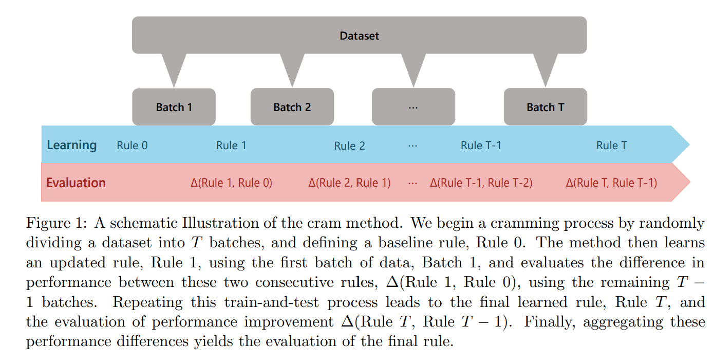
This procedure ensures each update is backed by performance testing, enabling both learning and evaluation in one pass over the data.

 

Note: this schematic represents how Cram estimates the difference in policy value (see the definition of policy value above) relative to a baseline policy - an example of baseline policy in healthcare would be to treat nobody (all-zeros) or to randomly treat individuals (assign 1 for treatment and 0 for no treatment randomly); the policy value difference “Delta” gives you how much better (or worse) is the policy learned by Cram on the data relative to the baseline policy - but Cram can also be used to estimate the policy value of the learned policy directly, without the need to specify a baseline policy (not presented here as part of the introduction but available in the outputs of the main functions of Cram; see result table below).

The cram_policy() Function

The cram_policy() function in cramR implements the Cram framework for binary treatment policy learning.

🔑 Key Features of cram_policy()

• Model-Agnostic Flexibility: Supports a variety of learning strategies, including causal_forest, s_learner, and m_learner, as well as fully customizable learners via user-defined fit and predict functions.

• Efficient by Design: Built on top of data.table for fast, memory-efficient computation, with optional support for parallel batch training to scale across larger datasets.

Example: Running Cram Policy on simulated data

library(data.table)
# Function to generate sample data with heterogeneous treatment effects:
# - Positive effect group
# - Neutral effect group
# - Adverse effect group
generate_data <- function(n) {
  X <- data.table(
    binary = rbinom(n, 1, 0.5),                 # Binary variable
    discrete = sample(1:5, n, replace = TRUE),  # Discrete variable
    continuous = rnorm(n)                       # Continuous variable
  )

  # Binary treatment assignment (50% treated)
  D <- rbinom(n, 1, 0.5)

  # Define heterogeneous treatment effects based on X
  treatment_effect <- ifelse(
    X[, binary] == 1 & X[, discrete] <= 2,        # Group 1: Positive effect
    1,
    ifelse(X[, binary] == 0 & X[, discrete] >= 4, # Group 3: Adverse effect
           -1,
           0.1)                                   # Group 2: Neutral effect
  )

  # Outcome depends on treatment effect + noise
  Y <- D * (treatment_effect + rnorm(n, mean = 0, sd = 1)) +
    (1 - D) * rnorm(n)

  return(list(X = X, D = D, Y = Y))
}

# Generate a sample dataset
set.seed(123)
n <- 1000
data <- generate_data(n)
X <- data$X
D <- data$D
Y <- data$Y

# Options for batch:
# Either an integer specifying the number of batches or a vector/list of batch assignments for all individuals
batch <- 20

# Model type for estimating treatment effects
# Options for model_type: 'causal_forest', 's_learner', 'm_learner'
# Note: you can also set model_type to NULL and specify custom_fit and custom_predict to use your custom model
model_type <- "causal_forest"  

# Options for learner_type:
# if model_type == 'causal_forest', choose NULL
# if model_type == 's_learner' or 'm_learner', choose between 'ridge', 'fnn' and 'caret'
learner_type <- NULL  

# Baseline policy to compare against (list of 0/1 for each individual)
# Options for baseline_policy:
# A list representing the baseline policy assignment for each individual.
# If NULL, a default baseline policy of zeros is created.
# Examples of baseline policy: 
# - All-control baseline: as.list(rep(0, nrow(X))) or NULL
# - Randomized baseline: as.list(sample(c(0, 1), nrow(X), replace = TRUE))
baseline_policy <- as.list(rep(0, nrow(X)))  

# Whether to parallelize batch processing (i.e. the cram method learns T policies, with T the number of batches.
# They are learned in parallel when parallelize_batch is TRUE
# vs. learned sequentially using the efficient data.table structure when parallelize_batch is FALSE, recommended for light weight training).
# Defaults to FALSE.
parallelize_batch <- FALSE  
 

# Model-specific parameters (more details in the article "Cram Policy part 2")
# Examples: NULL defaults to the following:
# - causal_forest: list(num.trees = 100)
# - ridge: list(alpha = 1)
# - caret: list(formula = Y ~ ., caret_params = list(method = "lm", trControl = trainControl(method = "none")))
# - fnn (Feedforward Neural Network): see below
# input_shape <- if (model_type == "s_learner") ncol(X) + 1 else ncol(X)
# default_model_params <- list(
#       input_layer = list(units = 64, activation = 'relu', input_shape = input_shape),
#       layers = list(
#         list(units = 32, activation = 'relu')
#       ),
#       output_layer = list(units = 1, activation = 'linear'),
#       compile_args = list(optimizer = 'adam', loss = 'mse'),
#       fit_params = list(epochs = 5, batch_size = 32, verbose = 0)
#     )
model_params <- NULL  


# Significance level for confidence intervals (default = 95%)
alpha <- 0.05  

# Run the Cram policy method
result <- cram_policy(
  X, D, Y,
  batch = batch,
  model_type = model_type,
  learner_type = learner_type,
  baseline_policy = baseline_policy,
  parallelize_batch = parallelize_batch,
  model_params = model_params,
  alpha = alpha
)

# Display the results
print(result)
#> $raw_results
#>                        Metric   Value
#> 1              Delta Estimate 0.23208
#> 2        Delta Standard Error 0.05862
#> 3              Delta CI Lower 0.11718
#> 4              Delta CI Upper 0.34697
#> 5       Policy Value Estimate 0.21751
#> 6 Policy Value Standard Error 0.05237
#> 7       Policy Value CI Lower 0.11486
#> 8       Policy Value CI Upper 0.32016
#> 9          Proportion Treated 0.60500
#> 
#> $interactive_table
#> 
#> $final_policy_model
#> GRF forest object of type causal_forest 
#> Number of trees: 100 
#> Number of training samples: 1000 
#> Variable importance: 
#>     1     2     3 
#> 0.437 0.350 0.213

Interpreting Results

result$raw_results
#>                        Metric   Value
#> 1              Delta Estimate 0.23208
#> 2        Delta Standard Error 0.05862
#> 3              Delta CI Lower 0.11718
#> 4              Delta CI Upper 0.34697
#> 5       Policy Value Estimate 0.21751
#> 6 Policy Value Standard Error 0.05237
#> 7       Policy Value CI Lower 0.11486
#> 8       Policy Value CI Upper 0.32016
#> 9          Proportion Treated 0.60500

result$interactive_table

The output of cram_policy() includes:

• raw_results: A data frame summarizing key evaluation metrics:

  • Delta Estimate: The estimated policy value difference i.e. improvement in outcomes from using the final learned policy compared to a baseline (e.g., no treatment or treat-all).
    
  • Delta Standard Error and confidence interval bounds: Reflect the uncertainty around the delta estimate.
    
  • Policy Value Estimate: The estimated policy value i.e. average outcome if the final learned policy were applied across the population.
    
  • Policy Value Standard Error and confidence interval bounds: Reflect uncertainty in the policy value estimate.
    
  • Proportion Treated: The fraction of the population that would be treated under the learned policy.

• interactive_table: A dynamic, scrollable version of raw_results for easier exploration and filtering.

• final_policy_model: The trained policy model object itself, fitted according to the specified model_type, learner_type, or user-provided custom_fit and custom_predict (more details in the article “Cram Policy part 2”). This object can be used for further analysis or for applying the learned policy to new data.

class(result$final_policy_model)
#> [1] "causal_forest" "grf"
summary(result$final_policy_model)
#>                          Length Class  Mode   
#> _ci_group_size              1   -none- numeric
#> _num_variables              1   -none- numeric
#> _num_trees                  1   -none- numeric
#> _root_nodes               100   -none- list   
#> _child_nodes              100   -none- list   
#> _leaf_samples             100   -none- list   
#> _split_vars               100   -none- list   
#> _split_values             100   -none- list   
#> _drawn_samples            100   -none- list   
#> _send_missing_left        100   -none- list   
#> _pv_values                100   -none- list   
#> _pv_num_types               1   -none- numeric
#> predictions              1000   -none- numeric
#> variance.estimates          0   -none- numeric
#> debiased.error           1000   -none- numeric
#> excess.error             1000   -none- numeric
#> seed                        1   -none- numeric
#> num.threads                 1   -none- numeric
#> ci.group.size               1   -none- numeric
#> X.orig                   3000   -none- numeric
#> Y.orig                   1000   -none- numeric
#> W.orig                   1000   -none- numeric
#> Y.hat                    1000   -none- numeric
#> W.hat                    1000   -none- numeric
#> clusters                    0   -none- numeric
#> equalize.cluster.weights    1   -none- logical
#> tunable.params              7   -none- list   
#> has.missing.values          1   -none- logical

You can inspect or apply the learned model to new data.

Visual Summary and Notes

 

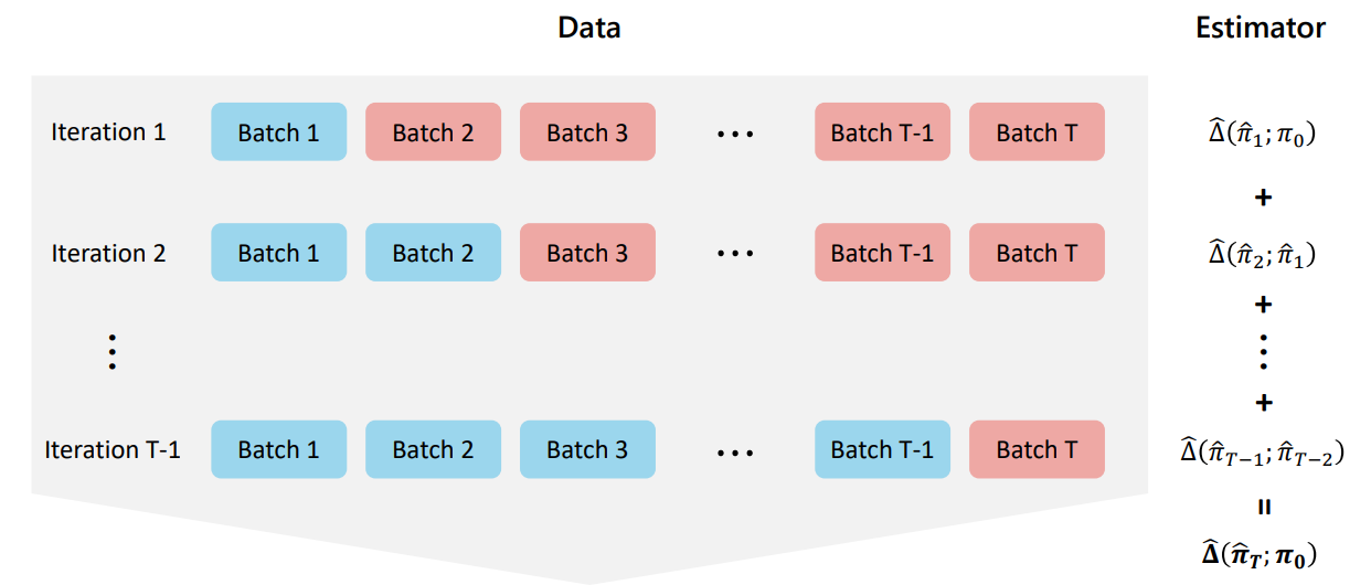
This visualization summarizes how multiple evaluations across iterations contribute to the full Cram estimate.

Notes:

• Batching: You can pass a number (e.g., batch = 5) or a custom vector to control how data is split.
  
• Parallelization: Enable with parallelize_batch = TRUE.
  
• Custom Learners: Use custom_fit and custom_predict to plug in any estimator. (more details in the article “Cram Policy part 2”)

📐 Comparing Evaluation Strategies: Sample-Splitting, Cross-Validation, and Cram

In this section, we compare classical strategies for model evaluation—namely sample-splitting and cross-validation—with the Cram method. While all three approaches may ultimately train a model using the full dataset, they differ fundamentally in how they estimate the generalization performance of that model.

🔍 Sample-Splitting

Sample-splitting divides the data into a training set and a held-out test set (e.g., 80/20). The model is trained on the training portion, and its performance is assessed on the held-out set. This procedure produces an evaluation of a model that was not trained on all the data, which may understate the performance of the final model trained on the full dataset. Thus, the evaluation corresponds to:

• A partially trained model (fit on, say, 80% of the data),
• Evaluated on unseen data (the held-out 20%).

This raises two issues:

• The model being evaluated is not the final model we would deploy (it’s undertrained).
• The evaluation uses only part of the available data, reducing statistical efficiency.

🔄 Cross-Validation

We consider k-fold cross-validation, which partitions the data into k equal-sized folds. For each fold, a model is trained on the remaining k-1 folds and evaluated on the held-out fold. This process ensures that each observation is used for both training and evaluation, but in different models. The final performance estimate is the average of fold-specific evaluation metrics and serves as a proxy for the expected performance of the model that would be trained on the full dataset.

• Each model is trained on a subset of the data (e.g., 4 folds out of 5),
• Evaluation is performed over the entire dataset, but using different models for each portion.

Thus, while cross-validation uses all data for evaluation, it only evaluates models trained on partial data. Crucially, the final model trained on the full dataset is never evaluated directly; its performance is approximated by averaging over surrogate models trained on subsets.

📈 Cram

Cram departs from these approaches by directly targeting the performance of the final model trained on the entire dataset, casting evaluation as a statistical estimation problem: it estimates the population-level performance (e.g., expected outcome or loss) that the model would achieve if deployed.

Specifically:

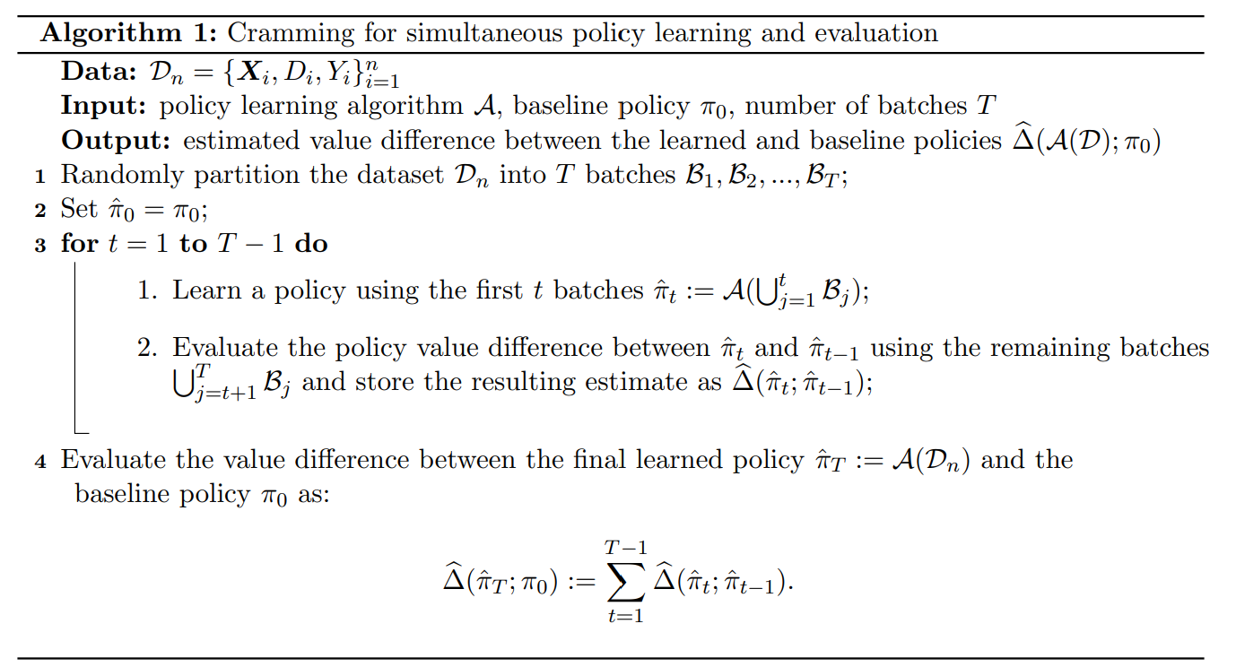
• Cram trains a sequence of models on cumulative batches and evaluates each on the remaining data, as described in Algorithm 1,
• Then uses statistical estimators to estimate the expected performance of the final model trained on the entire dataset—i.e., the outcome we would observe if this model were deployed at the population level beyond the observed sample,
• It provides confidence intervals around this estimate, which quantify uncertainty: for example, a 95% confidence interval is constructed such that, under repeated samples from the same data-generating process, the interval would contain the true expected performance in 95% of cases.

🧠 Key Distinction Summary: What Is Being Evaluated?

All methods aim to estimate the generalization performance of the model trained on the full dataset (denoted as final model in the table below for readability). However, they differ in the models trained during evaluation, the data used for evaluation, and how the final performance estimate is constructed.

Method	Evaluation Models Trained	Evaluation Data Used	Evaluation Mechanism
Sample-Splitting	One model trained on a subset	Held-out subset	Empirical performance on test set
Cross-Validation	k models trained on different subsets	Entire data (across folds)	Average of fold-specific evaluation metrics
Cram	Sequence of models trained on cumulative batches	Entire data	Statistical estimation of generalization performance of final model; provides confidence intervals and inference

final model*: model trained on the full dataset

• Sample-splitting trains a single model on a subset of the data and evaluates it on a held-out portion. This is simple but statistically inefficient.
• Cross-validation trains multiple models, each on a subset of the data, and evaluates each on its corresponding held-out fold. The fold-specific evaluation metrics are then averaged to approximate the final model’s performance. Although commonly used as a proxy for the generalization performance of the final model, this average does not directly target or estimate the performance of the model trained on the full dataset.
• Cram trains models on cumulative data batches and evaluates each on the remaining data. It uses these evaluations to statistically estimate the generalization performance of the final model trained on all data, providing both a point estimate and valid confidence intervals for the expected performance if deployed.

References

• Jia, Z., Imai, K., & Li, M. L. (2024). The Cram Method for Efficient Simultaneous Learning and Evaluation, URL: https://www.hbs.edu/ris/Publication%20Files/2403.07031v1_a83462e0-145b-4675-99d5-9754aa65d786.pdf.
  
• Künzel, S. R., Sekhon, J. S., Bickel, P. J., & Yu, B. (2019). Metalearners for estimating heterogeneous treatment effects using machine learning. Proceedings of the National Academy of Sciences of the United States of America, 116(10), 4156–4165. https://doi.org/10.1073/pnas.1804597116
• Wager, S., & Athey, S. (2018). Estimation and inference of heterogeneous treatment effects using random forests. Journal of the American Statistical Association, 113(523), 1228-1242.
• Athey, S., & Imbens, G. (2016). Recursive partitioning for heterogeneous causal effects. Proceedings of the National Academy of Sciences, 113(27), 7353-7360.